Poisson regression is used to predict a dependent variable that consists of "count data" given one or more independent variables. It shows how many times an event is likely to occur within a specific period of time.
Count Data Examples
The Number of Motorcycle Facilities in NCR Region
The Number of AIDS Cases LGBT Group
The Number of Persons killed in Typhoon Ondoy
Number of infected plants per transect
Forecasting Number of child abuse in a Year
The Number of Students Award with DOST Scholarship
Understanding Poisson Regression
A Poisson regression can be used to estimate how likely it is that something will happen “x” number of times. For example, if the average number of students who are enrolled in Medicine from the year 2017-2019 is 320, a Poisson Regression can answer the question, “What is the probability that more than 320 students will enroll in 2020?
Assumptions
The dependent variable consists of count data.
There are one or more independent variables which can be measured in a continuous, ordinal or nominal/dichotomous scale.
There must be independence of observations.
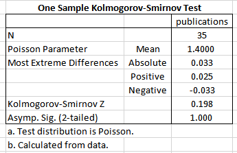
The distribution of counts follows a Poisson distribution.
The mean and variance of the model are identical.
Sample Research
The Director of Research of a small university wants to assess whether the rank of the professor and the time they have available to carry out research influence the number of publications they produce. Therefore, a random sample of 35 professors from the university is asked to take part in the research: 18 are associate professors and 17 are assistant professors. The number of hours they spent on research in the last 12 months and the number of peer-reviewed publications they generated was recorded.
The mean and variance of the model are identical.
The distribution of counts (conditional on the model) follows a Poisson distribution.
The first table in the output is the Model Information table (as shown below). This confirms that the dependent variable is the "Number of Publications", the probability distribution is "Poisson" and the link function is the natural logarithm (i.e., "Log").
The second table, Case Processing Summary, shows how many cases (e.g., subjects) were included in the analysis (the "Included" row) and how many were not included (the "Excluded" row), as well as the percentage of both.
The Categorical Variable Information table highlights the number and percentage of cases (e.g., subjects) in each group of each independent categorical variable in the analysis. In this analysis, there is only one categorical independent variable (also known as "factor"), which is the professorial rank.
The Continuous Variable Information table can provide a rudimentary check of the data for any problems but is less useful than other descriptive statistics that can be analyzed separately before running the Poisson regression.
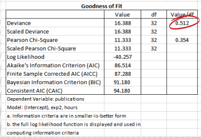
The Goodness of Fit table provides measures that can be used to assess how well the model fits. A value of 1 indicates equidispersion whereas values greater than 1 indicate overdispersion and values below 1 indicate underdispersion.
-overdispersed models more often indicate the usage of negative binomial
-under dispersed models more often indicates the usage of Poisson.
The Omnibus Test table fits somewhere between this section. It is a likelihood ratio test of whether all the independent variables collectively improve the model over the intercept-only model (i.e., with no independent variables added).
We can see that the professorial rank (exp2) is not statistically significant (p = .267), but the number of hours of work per week is statistically significant (p = .012). This table is mostly useful for categorical independent variables because it is the only table that considers the overall effect of the categorical variable in the study.
Poisson regression was used to predict the number of professors who published their research in peer-reviewed journals in the last 12 months based on professorial rank and the number of hours a professor spends each week working on research.
Based on the table, it means that the number of publications (i.e., the count of the dependent variable) will be 1.085 times greater for each extra hour of work per week. Another way of saying this is that there is an 8.5% increase in the number of publications for each extra hour of work per week.


No comments:
Post a Comment
Be sure to check back again because I do make an effort to reply to your comments here.